The Lifecycle of a ZK Proof

Over the last few blog posts, we’ve covered the fundamental math and cryptography concepts underlying zero-knowledge proofs (ZKPs). Now, we’ll see how they all fit together in the ZKP system.

So, if you haven’t read the previous posts, you’ll want to do that first. Here’s what you need to know:

• What the Heck is a Zero-Knowledge Proof, Anyway?
• You Can't Understand ZKPs Without Understanding Polynomials
• Why We Use Modular Math for Zero-Knowledge Proofs
• What are proof systems?

Let’s get started.

The Architecture of a Zero-Knowledge Proof System

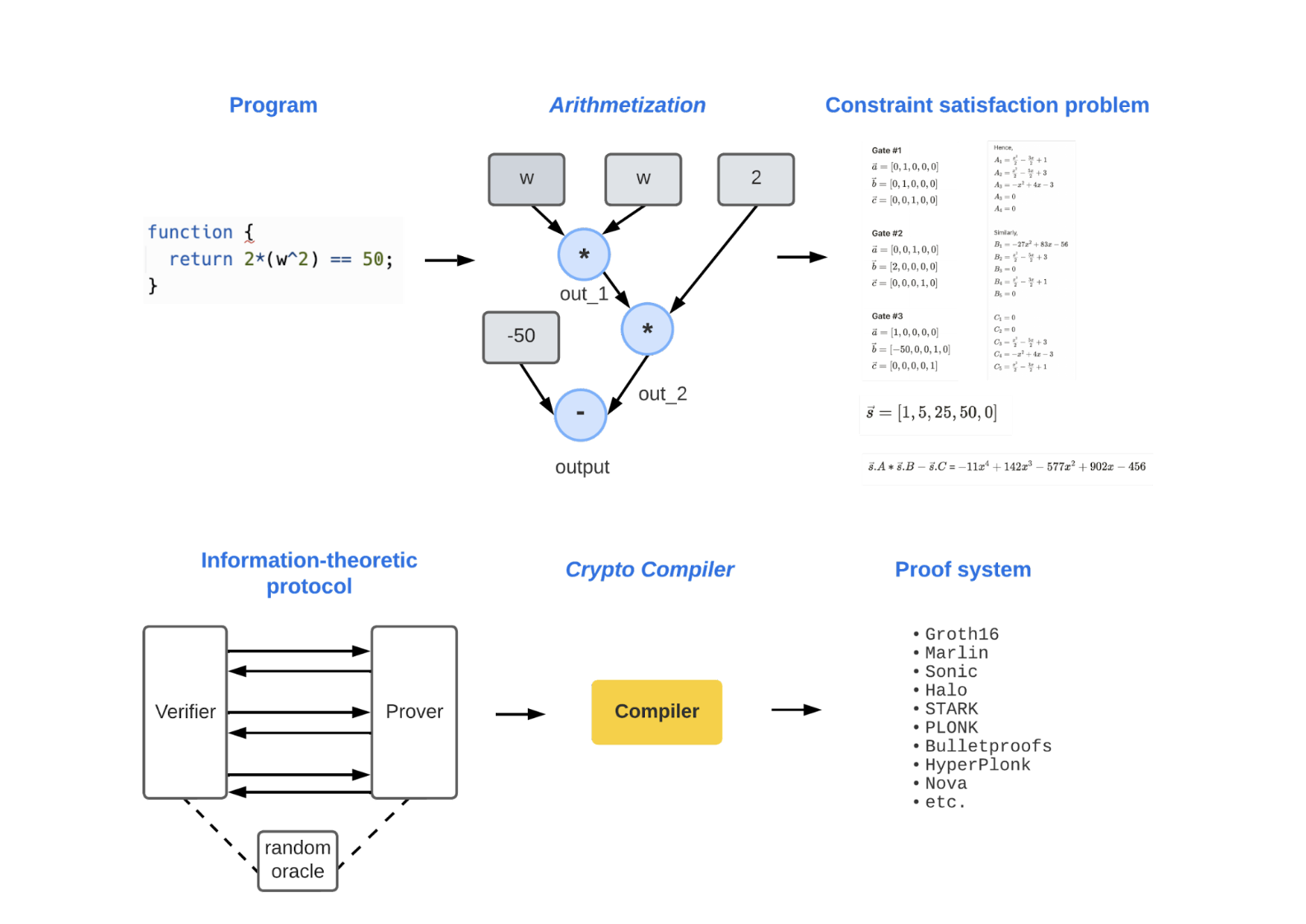
Here’s a diagram of how ZKPs are constructed. Take it all in! We’ll break down each part over the next few sections.

Construction of ZKPs

1. Computation

Let’s revisit the definition of a zk-SNARK. The goal is to let a prover prove they know a secret input, w, without revealing w. To do this, we write a program that takes in the secret input along with other parameters and then generates an output that we can check against our expected output.

ZKP Flow

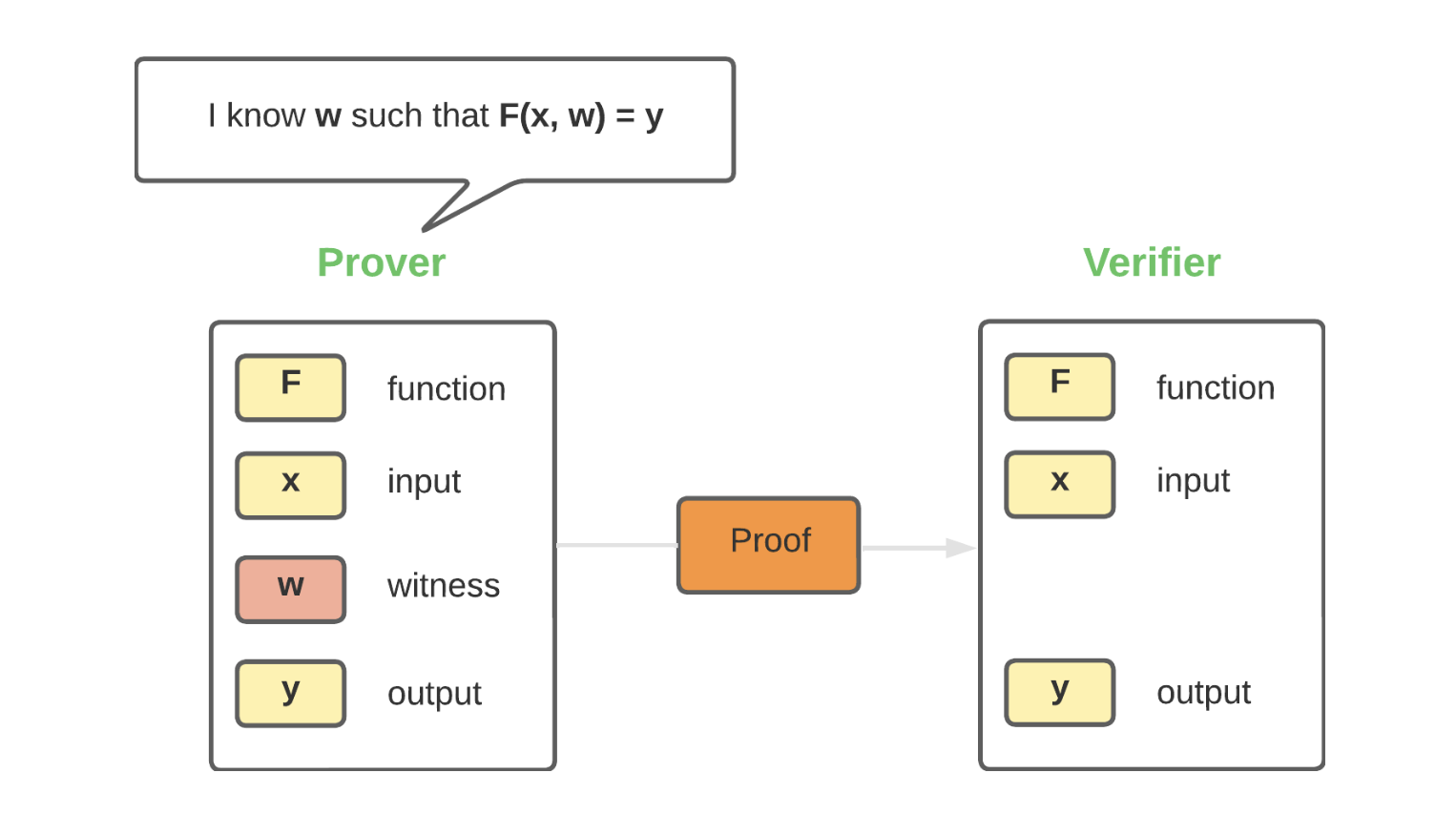
In short, we must be able to check the program’s output without revealing anything about the secret input. The first step of creating a proof system is defining this program. In our case, we’ll assume a very simple scenario:

Peggy (the prover) wants to prove to Victor (the verifier) that she knows some value w, which, when squared and doubled, equals 50. We can convert this scenario into a program:

$2*(w^2) \text{ == } 50;$

The program returns true if $2*(w^2)$ equals 50.

Now, this program is great, but we can’t really do much with it as it is. To generate a “proof,” we need to convert this program into something math-friendly. After all, a proof is a mathematical object, as we discussed in a previous post. This leads us to the next step: arithmetization.

2. Arithmetization

Arithmetization is the process of converting a program, which may contain arbitrarily complex statements and expressions, into a sequence of statements taking one of two forms:

$x = y$

$x = y [operator] z$

The operator can be addition or multiplication. So, we’re essentially taking the program and “flattening” it into a series of statements.

You can think of each statement as logic gates in a physical circuit.

Logic Gates

Source

Notice how each gate has two inputs and an output. Depending on the type of gate, the two inputs will be transformed into some output. For example, an AND gate with two inputs of 1 and 0, the output would be 0.

Similarly, we take the original program we defined in the computation step and turn it into a series of consecutive “gates.” This is called “flattening” because you’re literally flattening out the original program into logic gates.

Why do we do this? Because it lets us turn our program into a series of “constraints” that must be met. After all, a gate is simply an object that lets us define two inputs and the expected output. So, each “gate” represents a constraint, and the series of gates is a “circuit.”

Let’s put this into action. Using our example from above, we can envision the gates like this:

$out_1 = w * w$

$out_2 = out_1 * 2$

$output = out_2 - 50$

Once we convert our program into constraints, we can formulate a “Circuit Satisfaction Problem”, which we’ll describe next!

3. Circuit Satisfaction Problem

So, we just figured out how to define a set of constraints. Now, we need to ensure that those constraints are being met. This will let us check whether or not the output is what Peggy claims it is.

Enter: the circuit satisfaction problem (CSP)! Think of it like a mathematical object where the state of the object must satisfy several constraints. We’re simply checking that the constraints are met by turning our circuit into a math problem.

How does that work? Well, to create a CSP, we just take the circuit we defined in the last step and turn it into a polynomial. Using polynomials, we can check if all the constraints are being met — no matter how many there are! This is made possible by boiling them down into a polynomial equation, so we can check if they’re being met all at once.

Pretty neat, huh?

Going back to our example above, here’s what it looks if we convert our constraints into a CSP:

Gates:

$out_1 = w * w$

$out_2 = out_1 * 2$

$output = out_2 - 50$

Symbols:

$Symbols: [~one, w, out_1, out_2, output]$

Gate #1

$\vec{a} = [0, 1, 0, 0, 0]$

$\vec{b} = [0, 1, 0, 0, 0]$

$\vec{c} = [0, 0, 1, 0, 0]$

Gate #2

$\vec{a} = [0, 0, 1, 0, 0]$

$\vec{b} = [2, 0, 0, 0, 0]$

$\vec{c} = [0, 0, 0, 1, 0]$

Gate #3

$\vec{a} = [1, 0, 0, 0, 0]$

$\vec{b} = [-50, 0, 0, 1, 0]$

$\vec{c} = [0, 0, 0, 0, 1]$

$\vec{s} = [1, 5, 25, 50, 0]$

$\vec{a_1} = \begin{bmatrix} A_1(1) & A_2(1) & A_3(1) & A_4(1) & A_5(1) \end{bmatrix}$

$\vec{a_2} = \begin{bmatrix} A_1(2) & A_2(2) & A_3(2) & A_4(2) & A_5(2) \end{bmatrix}$

$\vec{a_3} = \begin{bmatrix} A_1(3) & A_2(3) & A_3(3) & A_4(3) & A_5(3) \end{bmatrix}$

Hence,

$A_1 = \frac{x^2}{2} - \frac{3x}{2} + 1$

$A_2 =$ $\frac{x^2}{2} - \frac{5x}{2} + 3$

$A_3 = -x^2 + 4x - 3$

$A_3 = 0$

$A_4 = 0$

Similarly,

$B_1 = -27x^2 + 83x - 56$

$B_2 = \frac{x^2}{2} - \frac{5x}{2} + 3$

$B_3 = 0$

$B_4 = \frac{x^2}{2} - \frac{3x}{2} + 1$

$B_5 = 0$

$C_1 = 0$

$C_2 = 0$

$C_3 = \frac{x^2}{2} - \frac{5x}{2} + 3$

$C_4 = -x^2 + 4x - 3$

$C_5 = \frac{x^2}{2} - \frac{3x}{2} + 1$

$\vec{s}.A* \vec{s}.B - \vec{s}.C$ = $-11x^4 + 142x^3 - 577x^2 + 902x - 456$

Explaining the math above is beyond the scope of this post, but stay tuned for an upcoming walkthrough!

4. Information-Theoretic Protocol

Now that we have a mathematical approach to verifying a solution, the next step is to figure out how the prover and verifier can interact to generate and verify the proof. This is called an “Information-Theoretic Protocol.”

We already discussed this protocol in a previous post on proof systems. There, we explained different types of proof systems, such as IP (Interactive Proof), PCP (Probabilistically Checkable Proof), and IOP (Interactive Oracle Proof). We also covered their assumptions about interaction and randomness, as well as their access to an oracle.

This is the step where we decide which assumptions to make when the prover and verifier interact. Once we have an information-theoretic proof system, all that’s left to do is use a crypto compiler to convert it into a real-world proof system.

5. Crypto Compiler

A crypto compiler removes the need for the idealized properties that an information-theoretic protocol makes. It’s pretty straightforward — crypto compilers use cryptography to “force” a prover and verifier to behave in a restricted manner. Because the prover and verifier act in a restricted (thus predictable) manner, we no longer have to assume ideal scenarios, such as having unbounded resources.

The output of the crypto compiler is a proof system with all the properties we’re seeking, such as zero-knowledge, succinctness, and non-interactivity.

Let’s look at a concrete example.

Example 1

An information-theoretic protocol may assume that the prover and verifier interact back and forth. In this case, the prover sends a “commitment” to some polynomial, the verifier sends a randomly generated “challenge” value to the prover, and then the prover computes the final proof based on both the commitment and challenge.

Instead of the verifier randomly generating and sending the challenge value to the prover, we can use an alternative like the Fiat-Shamir transformation, which lets the prover compute the value themselves by using a random function (such as a cryptographic hash function). Just keep in mind that figuring out the inputs to the hash function such that the proof can’t be forged can get tricky in practice.

Example 2

Let’s look at another example of how a crypto compiler removes idealized assumptions. An information-theoretic protocol may assume that we can trust the prover never to modify their proof based on questions from the verifier. Of course, in a real-world setting, this ideal assumption doesn’t work. This is where the cryptographic concept of a “commitment scheme” comes into play.

A commitment scheme lets a person “commit” to a chosen value or statement while keeping it hidden from others, with the ability to reveal the committed value later. The person can’t change the value or statement after they’ve committed to it. This means the commitment scheme is hiding (i.e., it hides the value) and binding (i.e., the value cannot be changed).

Therefore, the cryptographic compiler uses a commitment scheme to get rid of the assumption that an information-theoretic protocol makes about having a trusted prover.

Example 3

Let’s look at one last example. An information-theoretic protocol may assume that we have access to some random oracle that lets us generate perfectly random values that the verifier can use to challenge the prover. However, having access to a random oracle is not practical in a real-world setting, so a crypto compiler may, instead, add a “setup” phase where these random values are generated in advance.

Proof System

Here’s what we’ve been building up to! Once the information-theoretic protocol is transformed using a crypto compiler, we have a proof system. Viola!

Let’s take one last look at the proof system diagram. It should look a lot clearer to you now that you know how the pieces fit together.

Construction of ZKPs

“Front-End” vs. “Back-End”

Now that you understand how a proof system is constructed, we can roughly classify the first half as the “front-end” and the second half as the “back-end.”

Front-End v/s Back-End

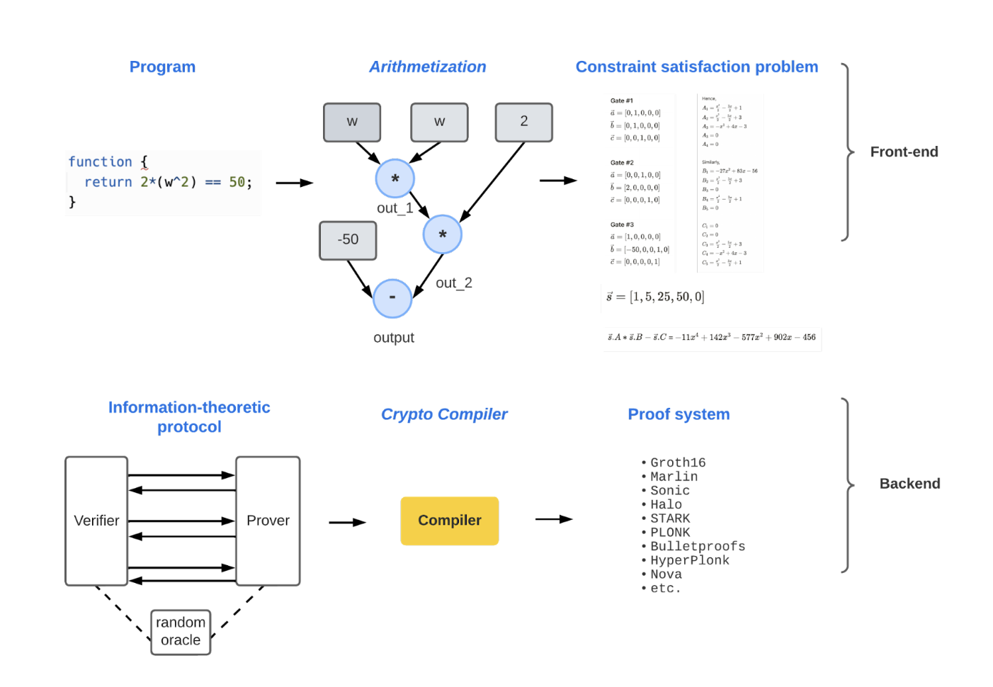
This distinction becomes really important once you realize that different tools and approaches are tailor-made for each end. More on that in future posts!

Until then, great work. Stay tuned!