Why we use Modular Math for Zero Knowledge Proofs
In the last article, we learned that zero-knowledge proofs (ZKPs) rely heavily on math. But those numbers can really get out of hand when we start generating ZKPs for large programs — even computers can start to break a sweat.
That’s where modular arithmetic comes in. Modular arithmetic, also known as clock arithmetic or modulo arithmetic, is a great fit for ZKPs due to its mathematical properties and computational efficiency. By using modular arithmetic, we unlock powerful capabilities like homomorphic encryption — which is key to the “hiding” features at the heart of ZKPs.
All of this and more in today’s post. Let’s start with the basics of modular arithmetic.
What is Modular Arithmetic
When we divide two integers, the equation looks something like this:
where R is the remainder.
Most of the time, we’re interested in the quotient (Q). But if you’re looking for the remainder (R), modular arithmetic is here to help.
We use the operator “modulus,” or “mod” as shorthand, when we want the remainder of dividing two numbers.
Here’s how that looks in action:
A mod B is ** R**
Let’s say A is 10 and B is 3. In that case, 10 mod 3 is 1.
Before we move on, there’s one important property of modulus that’s worth understanding. For any modulus, the remainder can be all integers ranging from 0 to n - 1 (where n is the modulus).
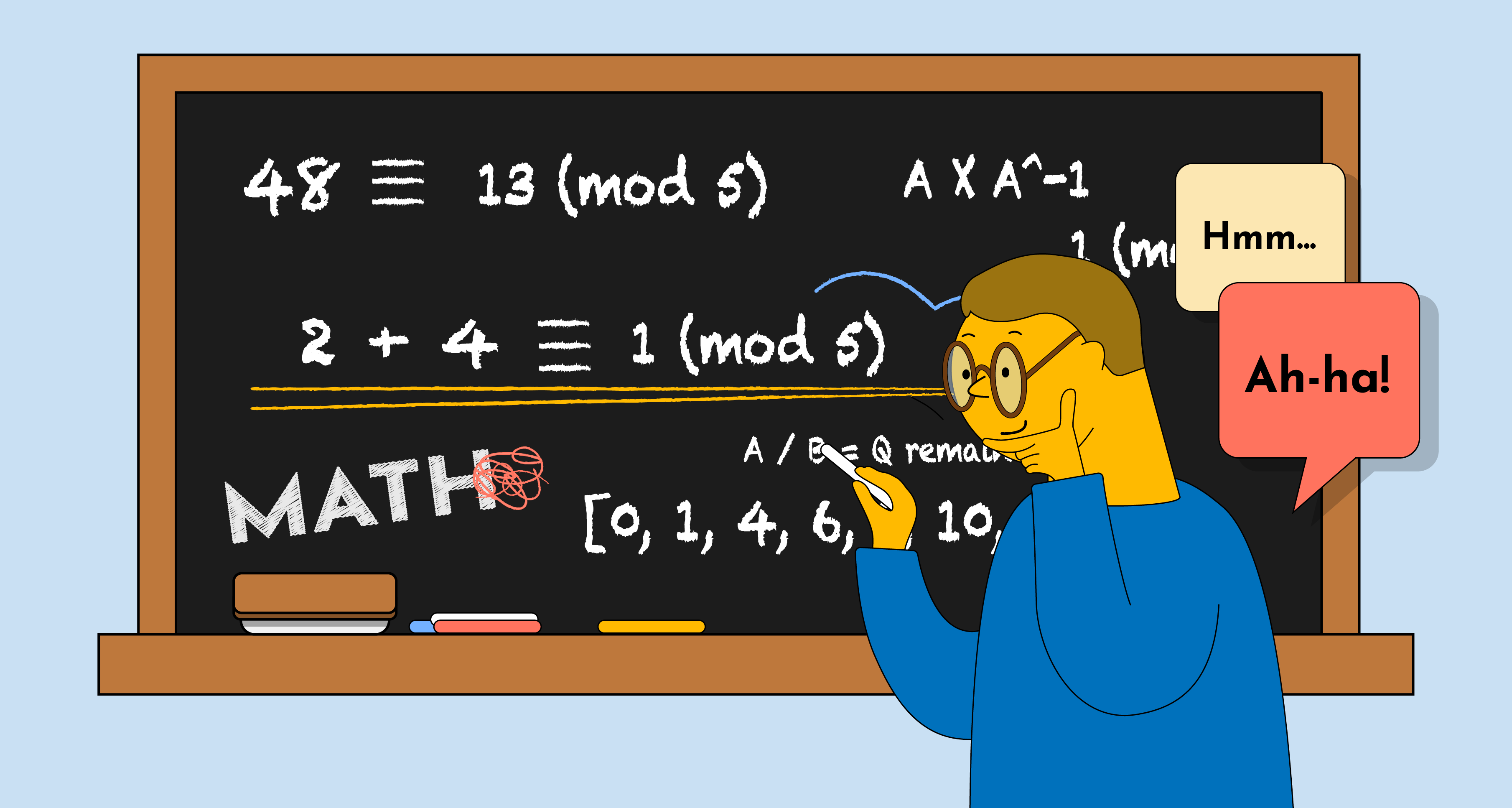
For example, for modulus 5, the possible remainders are 0, 1, 2, 3, and 4. So let’s say we have a set of integers [0, 1, 4, 6, 9, 10, 12, 18] and we do mod 5 on all of them. Due to this property, we know the resulting values will be [0, 1, 4, 1, 4, 0, 2, 3] — with each value falling within the range of 0 to 4.
Congruence
We’ll learn how to do modular math soon, but first, we need to learn an important notation: the ≡ operator.
The ≡ operator is called the “congruence” operator. It is NOT the same as the = equal operator that we’re all familiar with. Instead, ≡ has 3 vars and means that if we have two positive integers, a and b, then a and b are “congruent mod n” if the remainder when divided by n is the same.
For example:
48 divided by 5 gives us a remainder of 3. Similarly, 13 divided by 5 gives us a remainder of 3. Therefore, 48 and 13 are congruent mod 5.
Another example:
93 divided by 3 gives us a remainder of 0. Similarly, 6 divided by 3 gives us a remainder of 0. Therefore, 93 and 6 are congruent mod 3.
And that’s it! Now we’re ready for the math. Let’s take a look at how to perform addition, subtraction, multiplication, and division using modulus.
Addition
Adding in modular arithmetic is simple. We simply add the two numbers as usual, and then take the remainder when dividing by the modulus.
For example, 2 + 4 = 6 in regular arithmetic. But if we want 2 + 4 (mod 5), we get 1 as the remainder. So, we say that:
Notice how we used the congruence operator.
Subtraction
Subtracting in modular arithmetic follows the same logic. We simply subtract the two numbers as usual, and then take the modulus of the result. For example, 4 - 2 (mod 5) is 2 (mod 5) which is 2. So, we can write it as:
However, if we subtract the two numbers and get a negative number, then we add the modulus to the result until we get a non-negative answer that is less than the modulus.
For example, what is:
2 - 4 is -2, but we’re not allowed to have negative numbers. So we add 5 to it and get 3. 3 is non-negative and is our final answer. So we say that:
Multiplication
Now for multiplication in modular arithmetic. Simply multiply the two numbers as usual, and then take the remainder when dividing by the modulus. For example, 2 × 4 = 8, but in modular arithmetic with modulus 5, the remainder of 8 when divided by 5 is 3, so we say that:
Division
Curveball — there’s no division operation in modular arithmetic. But we do have modular inverses.
The modular inverse of
is
Therefore,
As we know, multiplying a number by the inverse of another is equivalent to dividing by that other number. For example:
Therefore, we can essentially “divide” some number “X” by another number “A” in Modular Math by first finding the multiplicative inverse of A and then multiplying X by this multiplicative inverse:
One important thing to note is that not all numbers will have a modular inverse. Only the numbers coprime to C (numbers that share no prime factors with C) have a modular inverse (mod C).
Now, how do we find the modular inverse? I encourage you to explore this on your own (hint: Learn more about Euclidean algorithm).
Three Reasons to Use Modular Arithmetic in ZKPs
Okay, so now that you understand the basics of modular math, you may be wondering how it’s useful for ZKPs. Let’s take a look.
1. Modular arithmetic works well with large numbers
When we perform arithmetic operations using modular arithmetic, the result of the operation is always between 0 and n - 1 (where n is the modulus). This gives us a nice, clean finite set of numbers to work with. That’s great because when we need to perform large numbers, we don’t have to worry about overflow issues.
This also prevents precision errors when we do division. Think about the regular method of divisions — sometimes, the results have decimal points. That can cause issues. It’s no wonder then why, with modular arithmetic, division also gives an element in the finite field so there are no precision errors to worry about.
2. Homomorphic properties
Modular arithmetic has homomorphic properties, which means certain operations can be performed on encrypted values without decrypting them. If you’re already drawing connections to the last post, good! These homomorphic properties enable the ZKP prover to perform operations and generate proofs without revealing the underlying values — an essential part of ZKPs.
3. Computational efficiency
Computations in modular arithmetic are typically faster than those involving real or rational numbers, as they only require integers within a fixed range. This makes modular arithmetic well-suited for resource-constrained environments, such as blockchain systems and embedded devices.
Conclusion
That’s all you need to know! Hopefully, this was a quick, painless, and helpful guide using modular arithmetic in Zero Knowledge Proof systems. For more detailed tutorials on modular math, I recommend the following resources: