You can't understand ZKPs without understanding polynomials
You know how data structures and algorithms are pretty much Computer Science 101? They’re fundamental to just about everything in the field. Well, polynomials are just as fundamental to zero knowledge proofs (ZKPs).
In case you need a primer, ZKPs let us prove a fact without revealing the fact. You can read my ZKP 101 post for all the details. But before we get into level 201, there’s a bit of math and cryptography we should cover.
In this blog post, we’ll focus on the math that makes ZKPs possible: Polynomials. Why? Because they’re really helpful in three major ways:
- They can encode an unbounded amount of data
- They can encode relationships between data
- They let us efficiently check whether two pieces of data are the same
Let’s get started with an overview!
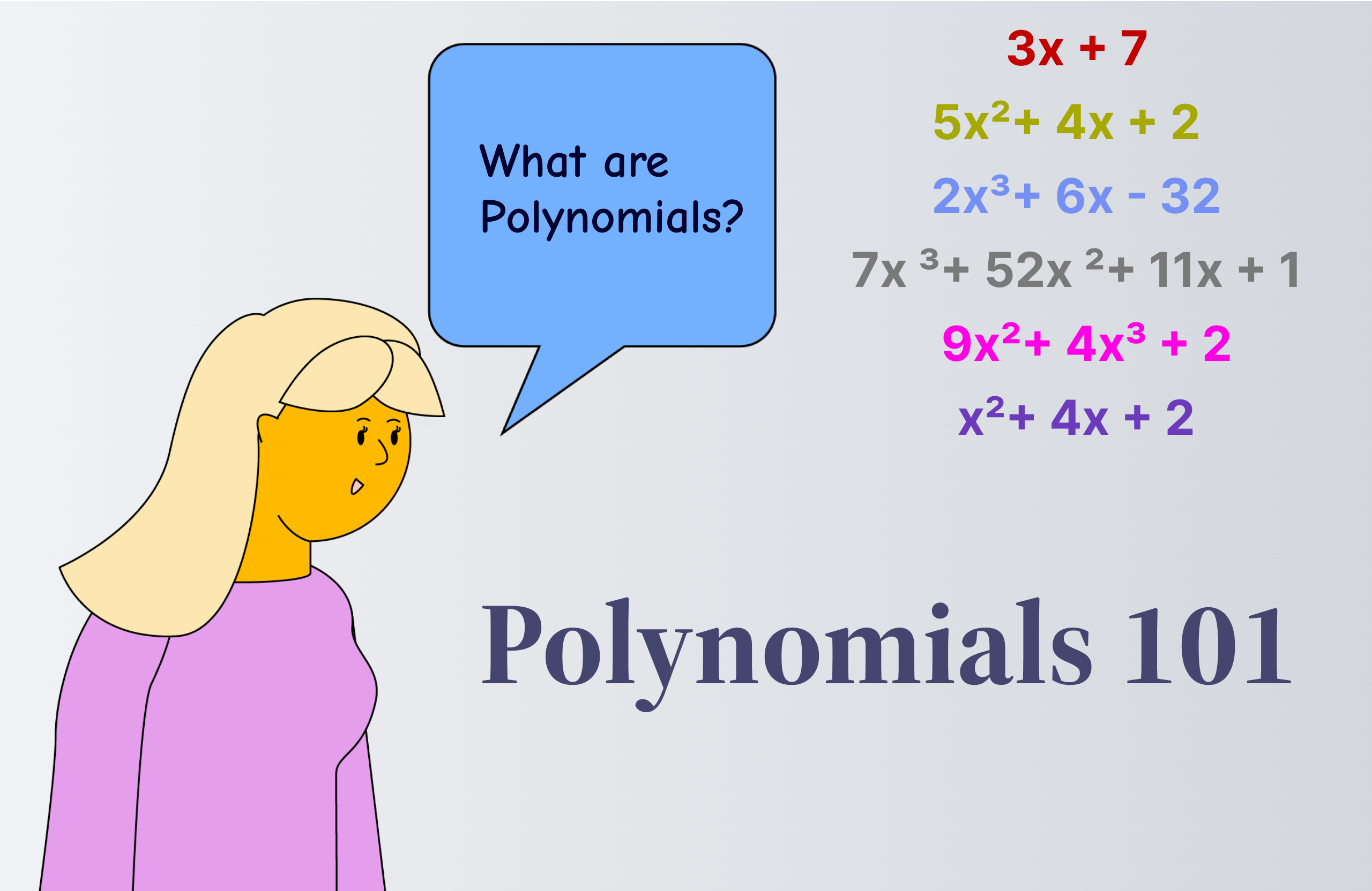
What are Polynomials?
Polynomials are mathematical expressions. Here’s what they look like:
You might be getting flashbacks to high school and college math classes. But don’t worry if you’ve forgotten everything about polynomials. We’ll go over everything you need to know. Let’s start with the most important terms.
Terminology
Degree
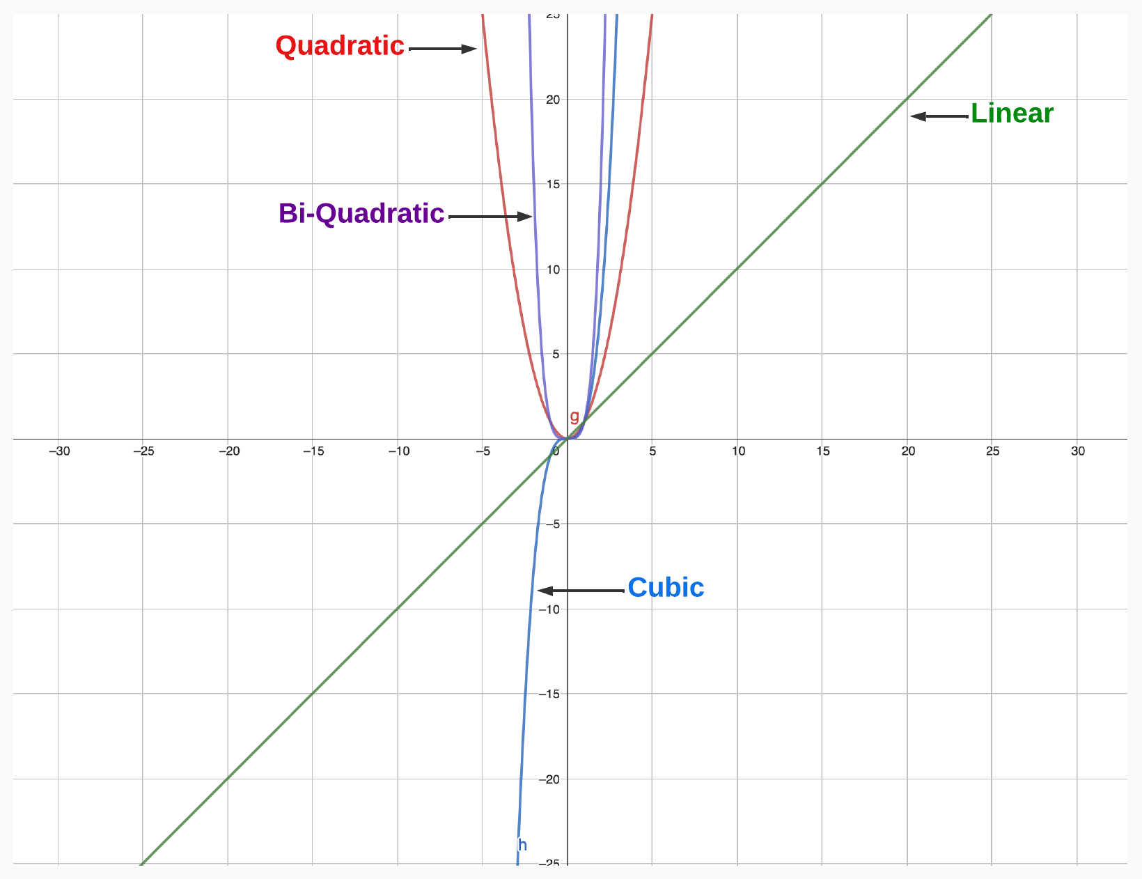
The degree of a polynomial is the highest power of the variable in the polynomial expression. For example, the polynomial above has a degree of 3 because the highest power of the variable x is 3.
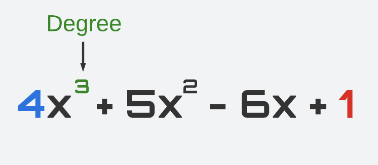
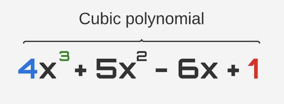
A polynomial of degree 1 (e.g., y = x) is called “linear.” A polynomial of degree 2 (e.g., y = x^2) is called a “quadratic” polynomial. A polynomial of degree 3 (e.g., y = x^3) is called a “cubic” polynomial. And so forth.
The degree of a polynomial determines its behavior and properties, such as its maximum or minimum values, the number of roots, and its symmetry.
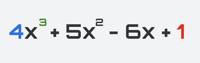
Coefficients
The coefficients of a polynomial are the numerical values that appear in front of each term. For example, in the polynomial below, the coefficients are 4, 5, -6, and 1.
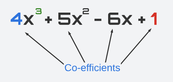
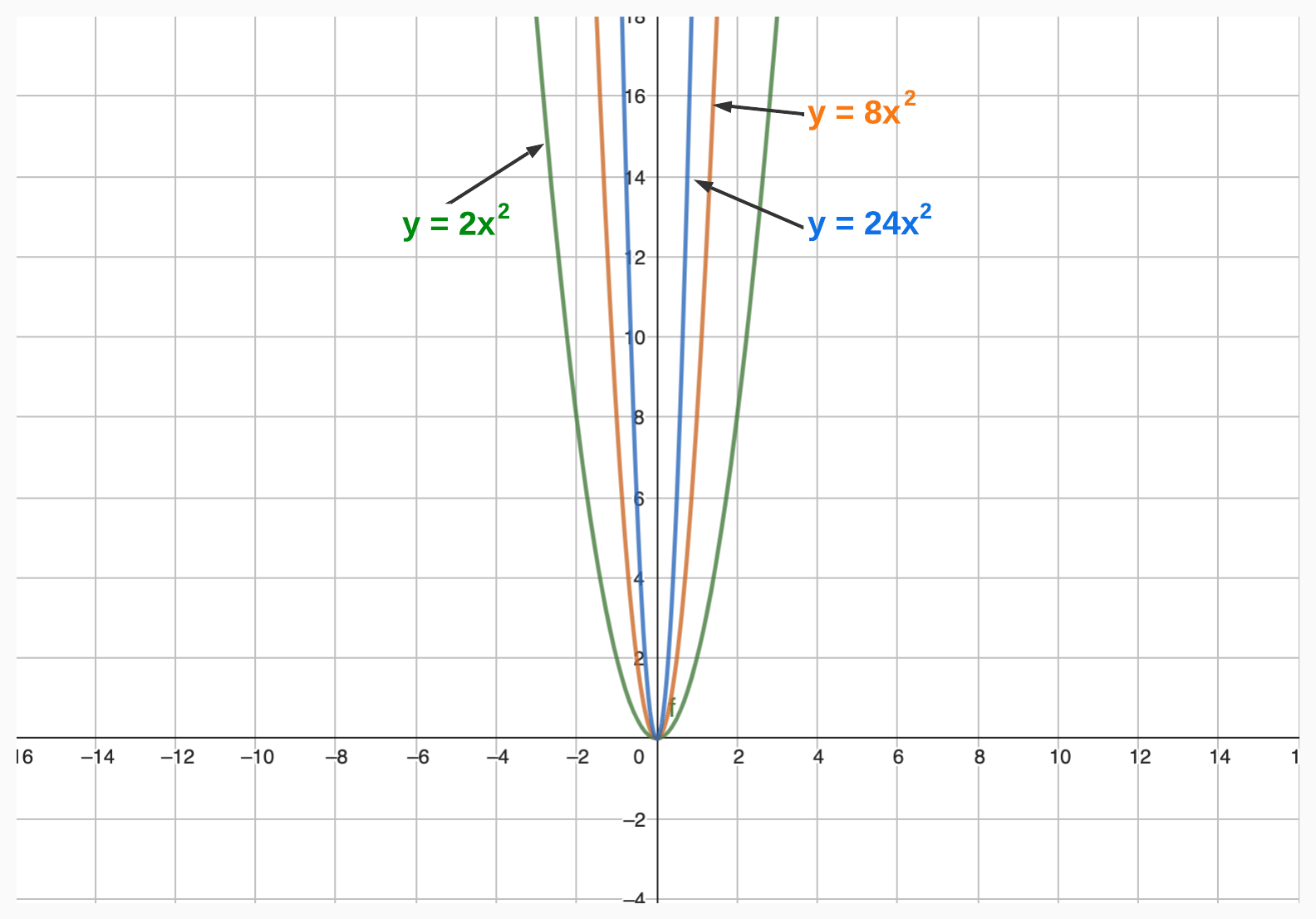
The coefficients determine the shape of the graph of the polynomial, including its height, width, and curvature.
Leading Coefficient
The leading coefficient of a polynomial is the coefficient of the term with the highest degree. For example, in the polynomial below, the leading coefficient is 4.
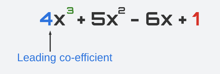
The leading coefficient is significant because it determines the end behavior of the polynomial–that is, the behavior of the graph as x approaches positive or negative infinity.
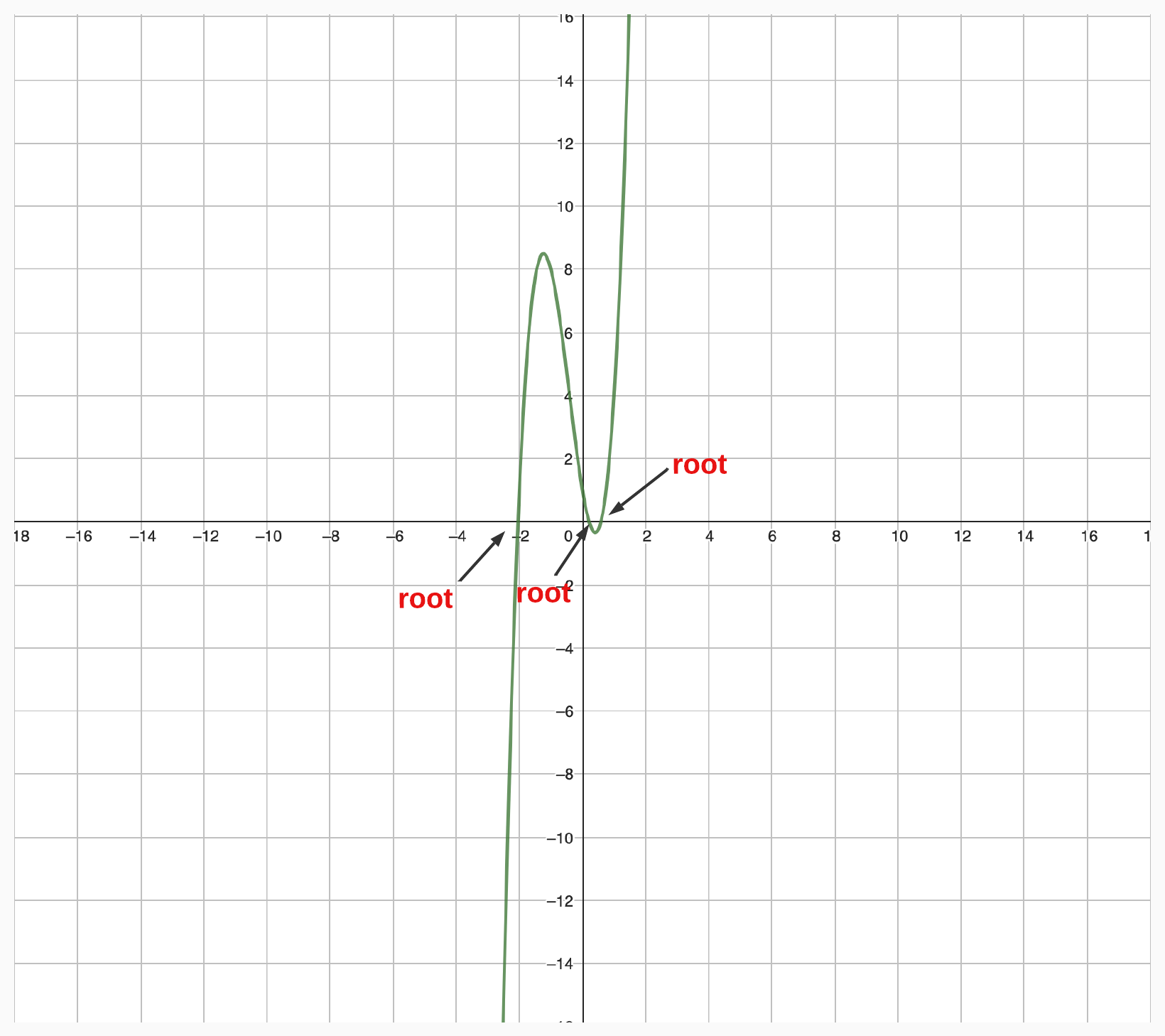
Roots
The roots of a polynomial are the values of the variable that make the polynomial equal to zero. For example, the roots of the polynomial
are the values of x that satisfy the following equation:
The roots of a polynomial are also called the “zeros,” “solutions,” or “x-intercepts” of the polynomial. The number of roots of a polynomial is equal to its degree.
Factorization
The factorization of a polynomial is the process of expressing it as a product of simpler polynomials. For example, the polynomial
can be factored as:
The factorization of a polynomial is useful because it can help us find its roots, simplify its expressions, and solve polynomial equations.
In this example, by factoring
...we can easily determine that 3 and -3 are roots of the polynomial. Try it yourself! Plug 3 and -3 into the expression.
Properties
Now that you have a grasp on the terminology of polynomials, let’s take a look at a few of their most fundamental properties.
Division Algorithm
If we divide the polynomial P(x) and the polynomial G(x) and get the polynomial Q(x) with a remainder of R(x), then we can write:
For example, if we have the polynomial
and we divide it by the polynomial
we get the quotient
and a remainder of 4.
Therefore, we can write P(x) as:
For more on how to divide polynomials, check out this link.
Factor Theorem
A polynomial P(x) is divisible by (x – a) if and only if P(a) = 0. In other words, if (x - a) is a factor of polynomial P(x), then P(a) = 0.
For example, if we have the polynomial
then (x - 3) and (x + 5) are both factors of the polynomial (ie. P(x) is divisible by (x - 3) and (x + 5)). You can check this by calculating P(3) and P(-5), and both will equal 0.
Remainder Theorem
If P(x) is divided by (x – a) with a remainder r, then P(a) = r.
For example, if we have the polynomial
and we divide it by (x - 3) (i.e., a = 3), then the quotient will be
and the remainder is -123.
Then, f(3) = -123.
Why are Polynomials Useful for ZKPs?
That’s it! You now have a grasp on the basics of polynomials. Now, let’s take a look at how these expressions can be used in action. We mentioned earlier that polynomials are useful for ZKPs for three reasons. Let’s take a look at those again:
- They can encode an unbounded amount of data
- They can encode relationships between data
- They let us efficiently check whether two pieces of data are the same
Let’s break down how each of these is made possible.
Polynomials Can Encode an Unbounded Amount of Data
Looks are deceiving. While polynomials might look like silly little equations, they can actually contain a lot of information. That’s because polynomials encode information via coefficients and exponents. So, each coefficient of a polynomial can represent a piece of information.
For example, if we have a number in its binary form, each coefficient of the polynomial can represent a binary digit. Therefore, if we have the number 1001 in its binary form, we can encode it as the polynomial:
Moreover, the degree of the polynomial tells us the amount of information being encoded.
For example, if we have a very large binary number 1 1000 0000 0000 0101, we can encode it as:
We see that the degree here is 16, implying a very large number.
Once we construct a polynomial that encodes our data, anyone can then recover the original data by evaluating the polynomial at specific points. These are handily known as “evaluation points.”
The binary example above is easy because we simply evaluate the polynomial by setting x = 2 to get the original number we started with. For example, we know that 1001 in binary form is equal to 9 in decimal form. And that’s exactly what we get when we plug in 2 into the polynomial
Let's try it:
So, why is this useful? Because we can even turn a large piece of code into a polynomial! It sounds insane, but it really is possible. And once we turn code into a polynomial, it’s in the right format to apply cryptography!
Polynomials Can Encode Relationship Between Data
Not only can we encode a lot of data within polynomials, but we can also encode relationships between data.
This process is called “polynomial interpolation,” which involves taking a set of data points and approximating a polynomial that passes through all of them. That special polynomial encodes the relationship between all of the data points. Let’s see how it works.
Polynomial Interpolation
Let’s say we have a set of points:
To find the special polynomial that passes through all of these points, we can use “Lagrange interpolation.”
Lagrange interpolation works by calculating the “basis” functions using the x-coordinates and then multiplying each basis function by the y value of that coordinate.
The formula looks like this:
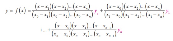
Sounds like a lot of jargon...but don't worry. It is simpler than it looks.
The best way to explain this is through an example.
Once we have the polynomial, we can then use it to interpolate the value of the function at any point within the range of data points. For example, we can now interpolate what the value will be if the x-coordinate is 10 by simply plugging 10 into the final polynomial, as seen below.
Polynomial interpolation is useful because it is one of the steps required to convert a large piece of code into polynomials. First, the code is converted into a series of “constraints.” For example:
And so on.
Now, we can represent these constraints as vectors and then use Lagrange interpolation to convert these vectors into polynomials. The result is our same large program, but now it’s compressed into polynomial format so that we can apply cryptography on.
Polynomials Let Us Efficiently Check Whether Two Pieces of Data are the Same
In a proof system, we encode hidden information that the prover knows into a polynomial. The tricky part is having the prover prove their knowledge of the secret polynomial without revealing it. To accomplish this, we simply check if the secret polynomial is equal to another polynomial that’s publicly known.
If they’re equal, then the prover knows the private polynomial. Don’t worry — this will make more sense in future posts, where we’ll get into the details. For now, just understand that we need to be able to check whether two polynomials are the same (or not). In other words, we need to conduct “polynomial identity testing.”
Let’s look at an example. How can we check whether
equals
First, we can move things around to ask the question in a slightly different way:
vs.
In other words, we need to figure out if
is identical to the zero polynomial (i.e., 0 is the zero polynomial).
There are several ways to do polynomial identity testing, including sheer brute force, where we test all values of x until we find something that gives us the 0 polynomial. But brute force is really inefficient, especially as the polynomials get larger.
That’s why we use an approach called the “Schwartz-Zippel” Lemma — think of it as a shortcut. Schwartz-Zippel Lemma states that the probability of a nonzero polynomial evaluating to zero at a random point is, at most, the degree of the polynomial divided by the number of possible evaluation points.
Another way to think about it is that there is a very small probability (almost negligible chance) that a polynomial that is NOT a zero polynomial will evaluate to zero if you picked a random point and evaluated it at that point.
Of course, this shortcut isn’t perfect. It only gives us a probabilistic guarantee, and as such, there will always be a tiny probability that we find a nonzero polynomial that evaluates to zero at a random point. But this probability gets smaller as the number of possible evaluation points increases. And since ZKP systems typically involve very large polynomials, the Schwartz-Zippel Lemma is good enough.
In short, we can check if two polynomials are equivalent by simply picking random points and evaluating the two polynomials at those points. If they’re equal at all the randomly chosen points, we know the polynomials are most likely the same.
Pretty neat, huh?
Conclusion
Kudos for making it to the end! Re-learning math as an adult can be daunting, but I promise it’s worth it. Better yet, taken one step at a time, you’ll find that it isn’t quite as challenging as it was back in math class.
That’s it! We’ve covered the majority of the math you’ll need to know. If there are parts that didn’t fully click, I encourage you to search online and see if you can find resources that explain that specific part.
In the next post, we’ll cover the basics of Modular Math and why we use it in zero knowledge proofs. See you then!